Link to contributors: Jason Van Der Byl, Trenton Harris, and Gray Huddleston

For our project, we used a global natural disasters data set covering 2018 to 2024. The data set includes records of disasters occurring worldwide and provides both geographic and impact/response-related variables. Key fields include: Date of disaster occurrence, Country affected, Disaster type (e.g., flood, earthquake), Severity index (numeric measure of disaster severity), Casualties (people affected or killed), Economic loss (USD), Response time (hours), Aid amount (USD), Response efficiency score (0–100), Recovery days, and Geographic latitude (and associated location fields such as longitude) This data set allowed our team to explore patterns in disaster frequency, location clustering, response performance, and recovery outcomes over time and across regions.

We then took this data to answer 4 questions with visualization aids:

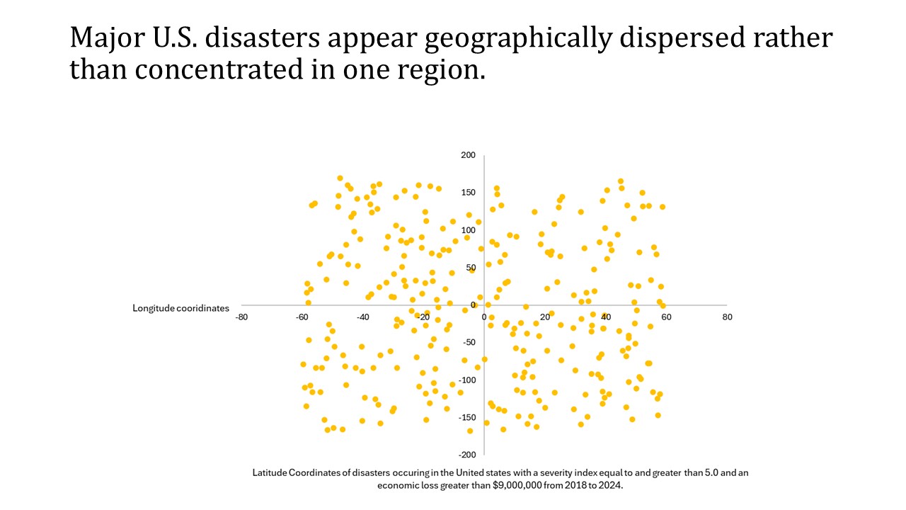
Is there a geographical pattern among disasters occuring in the United States?

This question was interesting to us because we wanted to see whether disasters in the United States show a meaningful geographic concentration. If disasters were clustered in specific regions, that could point toward geographic vulnerability, infrastructure risks, or environmental trends. Understanding whether disasters are concentrated or spread out also helps with planning, preparedness, and resource allocation.To make the visualization readable and meaningful, We narrowed the dataset to: Country = United States, Severity index > 5.0. This filtering step reduced the number of plotted points enough to create a clear scatter-based map-style display. This approach ensured we were focusing on stronger or more impactful disasters rather than overcrowding the chart with minor events. In Excel, this involved: Applying filters to the dataset (Country and Severity Index), Confirming that only U.S. records above the threshold remained, Selecting the geographic coordinate columns (Latitude and Longitude) for plotting. For the slide visual, we used a scatter plot: X-axis: Longitude, Y-axis: Latitude, Each point: A disaster event. By plotting latitude and longitude, we created a simple geographic distribution view of major U.S. disasters. The scatter plot format was the most direct way to show spatial spread without needing advanced mapping tools. After filtering to U.S. disasters with a severity index above 5.0, we found that disasters appear to occur randomly across the United States. There was no single dominant hotspot that clearly suffered more than another. Instead, the distribution suggested that major disasters are spread broadly across the country, rather than clustering in one specific region.

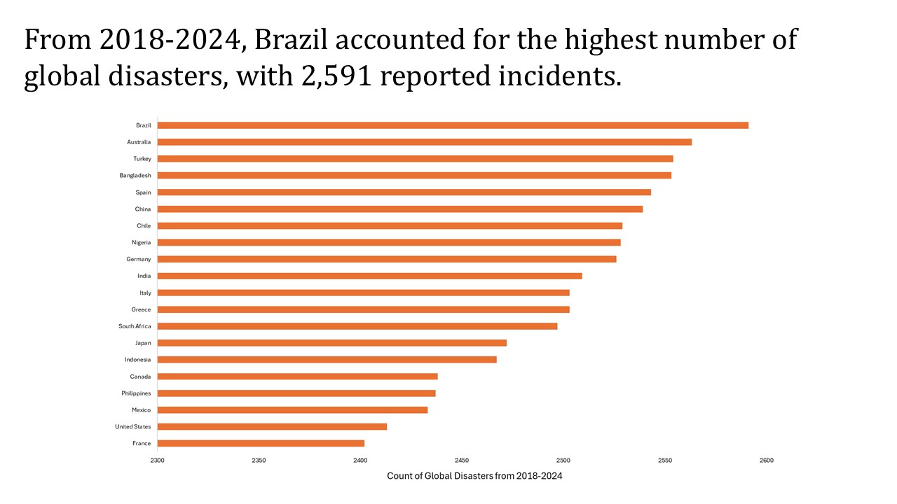
Which country experienced the most natural disasters?

This question was interesting to us because we wanted to better understand patterns among disasters. Disasters impact every country differently and it was interesting to see which countries were impacted the most. We wanted to not only find where most disasters occur, but also how many occur in each country. In excel we added a new column for the count of the disaster (1-50,000). With this new column, we were able to insert a pivot table that would make creating the graph much simpler. With the pivot table we were able to select the count and the country tabs. The pivot table gave us a table with each country listed in the data set and how many disasters occurred for each one. We decided a bar graph would best show which country experienced the most natural disasters and were able to create it with the numbers the pivot table gave us. The x-axis shows the count of disasters, and the y-axis shows each country in the data set. We found that Brazil experienced 2,591 disasters in a six-year period, which was the most among countries.

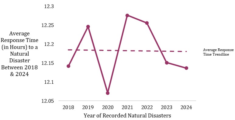
Has the average response time changed over the years?

We’re interested to see what change, if any, there has been over time because, theoretically, response time should improve over time as we improve our technologies and strategies. In Excel, we took the dataset and created a copy of it on a new worksheet. We then deleted all but the relevant columns to this question, for clarity. These columns were the date, response time, and year column (which we created using the “=Year()” function that took the date and output only the integer year). We then created a table to the right of the columns with each year listed (2018-2024) in the left column and the average response time in the right column. The data was averaged using an AVERAGEIF function, with the if condition column being our created year column, the condition being if the data point was in the given year, and the average column being the response time column. We then input this table into 2D Line Chart with the X-Axis being the Year and the Y-Axis being the Average Response Time. Lastly, we added a trendline to see where response time is trending. This trendline lead us to conclude that average response time remains negligibly changed over the years as the average change across years was -0.0007 hours (or 2.52 seconds a year in decreased response time). There was, however, a low amount of variability in the response time as the range on the averages was approximately 0.21 hours or 12.6 minutes (highest average was 12.28 hours for 2021 and lowest was 12.07 hours for 2020).

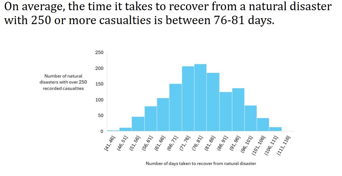
What is the average recovery days for natural disasters with 250 or more casualties?